2. Running an example simulation

2.1. Preparation

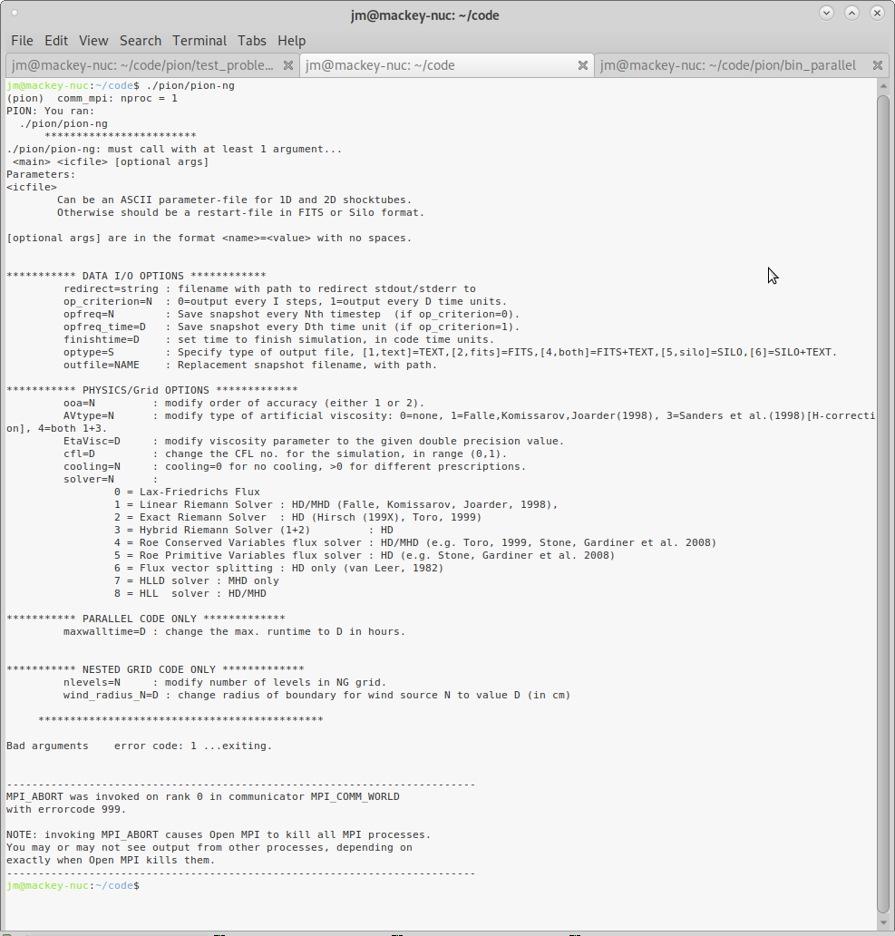
Fig. 2.1 Screenshot: running PION.

This simulation can be run on a workstation with only a few cores in less than an hour. Once you have obtained a copy of PION (we assume you installed into a directory called pion/) and compiled it following the instructions in Getting Started, so that you have the binary files pion/icgen-ng and pion/pion-ng on your system.

Test that these files run without library/system problems by running, e.g., $ ./pion/pion-ng and see what is displayed on screen. It should look like Fig. 2.1. Once you have verified this, then you can run a test simulation and view the results.

2.2. 2D simulation of a bow shock around a moving star

Change directory to the 2D bow-shock test directory:

$ cd pion/test_problems/Wind2D/

The parameters for the test simulation that we will run are in the file params_Wind2D_HD_l3n0128.txt. You can download the file here. Some of the key physical parameters are:

EP_cooling      8
...
UNIFORM_ambRO 7.0e-24   # Density in g/cm^3
UNIFORM_ambPG 7.0e-12   # Pressure in dyne/cm^2
UNIFORM_ambVX -25.0e5   # X-velocity of background medium
...
WIND_0_pos0  0.0e18   # X-position of Wind source
WIND_0_pos1  0.0e18   # Y-position of Wind source
WIND_0_pos2  0.0e18   # Z-position of Wind source
WIND_0_radius 2.0e17  # radius of boundary region: ~20 cells for 128^2, 3 levels
WIND_0_type   0       # Constant wind
WIND_0_mdot   1.0e-8  # mass-loss rate in solar masses per year
WIND_0_vinf   1500.0  # wind speed in km/s
WIND_0_vrot   200.0   # surface rotation in km/s
WIND_0_temp   3.0e4   # effective temperature in K
WIND_0_Rstr   1.0e12  # radius of surface in cm
WIND_0_Bsrf   0.0

This sets up a uniform interstellar medium (ISM) with the density, pressure and velocity given by the above parameters, and stellar-wind properties given below the ISM values. Radiative cooling flag, EP_cooling     8 uses a cooling function appropriate for photoionized gas, with strong heating that gives an gas equilibrium temperature around 7500K.

Execute the following commands to set the simulation running:

$ mpirun -np 2 ../../icgen-ng params_Wind2D_HD_l3n0128.txt
$ mpirun -np 4 ../../pion-ng Wind2D_HD_l3n0128_level00_0000.00000000.silo

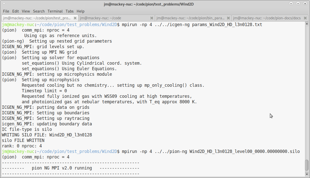
Fig. 2.2 Screenshot of setting up initial conditions.

The first command sets up the initial conditions (here using 2 MPI processes) and saves an initial snapshot in the current directory in SILO format. If the command worked, you should see some output like that shown in Fig. 2.2, and 3 silo files should be present:

jm@mackey-nuc:~/code/pion/test_problems/Wind2D$ ls -l Wind2D_HD_l3n0128_level0*.00000000.silo
-rw-r--r-- 1 jm jm 1064893 May 13 15:44 Wind2D_HD_l3n0128_level00_0000.00000000.silo
-rw-r--r-- 1 jm jm 1064893 May 13 15:44 Wind2D_HD_l3n0128_level01_0000.00000000.silo
-rw-r--r-- 1 jm jm 1064893 May 13 15:44 Wind2D_HD_l3n0128_level02_0000.00000000.silo

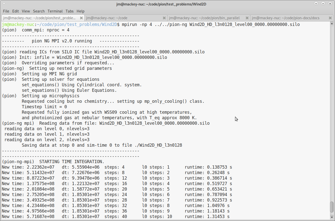
Fig. 2.3 Screenshot of running a 2D bow-shock simulation.

The second command calls pion-ng, running on 4 cores (MPI processes), with the level-0 data snapshot as the command-line argument. This runs the simulation, and you should see output on screen like in Fig. 2.3.

The simulation is set to run until \(t=3.156\times10^{12}\,\mathrm{s}\) (100,000 years), which takes about 184,000 timesteps and 2 hours wall-time to run to completion, saving snapshots every 1024 timesteps. You should see files start to appear in the current directory, e.g.,

jm@mackey-nuc:~/code/pion/test_problems/Wind2D$ ls Wind2D_HD_l3n0128_level0*.0000*
Wind2D_HD_l3n0128_level00_0000.00000000.silo  Wind2D_HD_l3n0128_level01_0000.00005120.silo
Wind2D_HD_l3n0128_level00_0000.00001024.silo  Wind2D_HD_l3n0128_level01_0000.00006144.silo
Wind2D_HD_l3n0128_level00_0000.00002048.silo  Wind2D_HD_l3n0128_level01_0000.00007168.silo
Wind2D_HD_l3n0128_level00_0000.00003072.silo  Wind2D_HD_l3n0128_level01_0000.00008192.silo
Wind2D_HD_l3n0128_level00_0000.00004096.silo  Wind2D_HD_l3n0128_level01_0000.00009216.silo
Wind2D_HD_l3n0128_level00_0000.00005120.silo  Wind2D_HD_l3n0128_level02_0000.00000000.silo
Wind2D_HD_l3n0128_level00_0000.00006144.silo  Wind2D_HD_l3n0128_level02_0000.00001024.silo
Wind2D_HD_l3n0128_level00_0000.00007168.silo  Wind2D_HD_l3n0128_level02_0000.00002048.silo
Wind2D_HD_l3n0128_level00_0000.00008192.silo  Wind2D_HD_l3n0128_level02_0000.00003072.silo
Wind2D_HD_l3n0128_level00_0000.00009216.silo  Wind2D_HD_l3n0128_level02_0000.00004096.silo
Wind2D_HD_l3n0128_level01_0000.00000000.silo  Wind2D_HD_l3n0128_level02_0000.00005120.silo
Wind2D_HD_l3n0128_level01_0000.00001024.silo  Wind2D_HD_l3n0128_level02_0000.00006144.silo
Wind2D_HD_l3n0128_level01_0000.00002048.silo  Wind2D_HD_l3n0128_level02_0000.00007168.silo
Wind2D_HD_l3n0128_level01_0000.00003072.silo  Wind2D_HD_l3n0128_level02_0000.00008192.silo
Wind2D_HD_l3n0128_level01_0000.00004096.silo  Wind2D_HD_l3n0128_level02_0000.00009216.silo

2.3. Looking at the results

Now you are running a simulation and want to see how the solution is evolving. You have at least two options, using python to read in the data and plotting with e.g. matplotlib, or using VisIt, software for visualizing scientific data from LLNL and freely available to download and install (but not included by default in most linux distributions).

We’ll describe using VisIt here, but there is more information on reading and plotting snapshots using python in this documentation [ADD LINK!] Here are the steps for plotting the simulation data with VisIt:

• Open level-0 data using the File->Open dialog.

• Add Pseudocolor plot of variable Density

• Open level-1 data using the File->Open dialog.

• Add Pseudocolor plot of variable Density

• Open level-2 data using the File->Open dialog.

• Add Pseudocolor plot of variable Density

• If a pop-up box asks if you want to create a database correlation, click yes. If not, then go to Controls->Database Correlations and create a new correlation between the three databases. This allows you to step all levels forward in time in sync with each other.

• Click Draw

• Open the PlotAtts->Pseudocolor dialog with all three plots selected in the Plots window.

• Change the scale to Log, and set Minimum and Maximum values to 1e-27 and 1e-23, respectively. Click Apply. This sets the plots for all 3 levels to use the same scale.

• You should be able to use the playback arrows on the GUI to step between different snapshots.

A python script that performs these steps can be downloaded from here and, when saved in the same directory as the silo snapshots, can be run via

jm@mackey-nuc:~/code/pion/test_problems/Wind2D$ visit -s visit_commands.py
Running: gui3.1.1 -s visit_commands.py
Running: viewer3.1.1 -s visit_commands.py -geometry 1379x971+541+56 -borders 31,6,6,6 -shift 6,31 -preshift 0,0 -defer -host mackey-nuc -port 5600
Running: mdserver3.1.1 -host 127.0.0.1 -port 5601
Running: xterm -geometry 120x40 -title "VisIt cli3.1.1" -e "/usr/local/visit/3.1.1/../bin/visit -cli -v 3.1.1 -reverse_launch -host 127.0.0.1 -port 5600 -key 25ab19f4f78d684151ff"
Running: mpirun -np 1 /usr/local/visit/3.1.1/linux-x86_64/bin/engine_par -plugindir /home/jm/.visit/3.1.1/linux-x86_64/plugins:/usr/local/visit/3.1.1/linux-x86_64/plugins -visithome /usr/local/visit/3.1.1 -visitarchhome /usr/local/visit/3.1.1/linux-x86_64 -host mackey-nuc -port 5600

Fig. 2.4 shows a screenshot of the gas density in the initial conditions for this simulation, using the above python script for setting the display parameters. The inner 75% of the wind boundary region is set to a very low density (\(10^{-31} \,\mathrm{g\,cm}^{-3}\)) and the outer 25% to the values appropriate for a freely expanding flow at the wind terminal velocity. The symmetry axis is the \(x\)-axis, which corresponds to \(\hat{z}\) in cylindrical coordinates, and the \(y\)-axis is the radial direction \(\hat{R}\). As such, the solution has rotational symmetry around the \(x\)-axis.

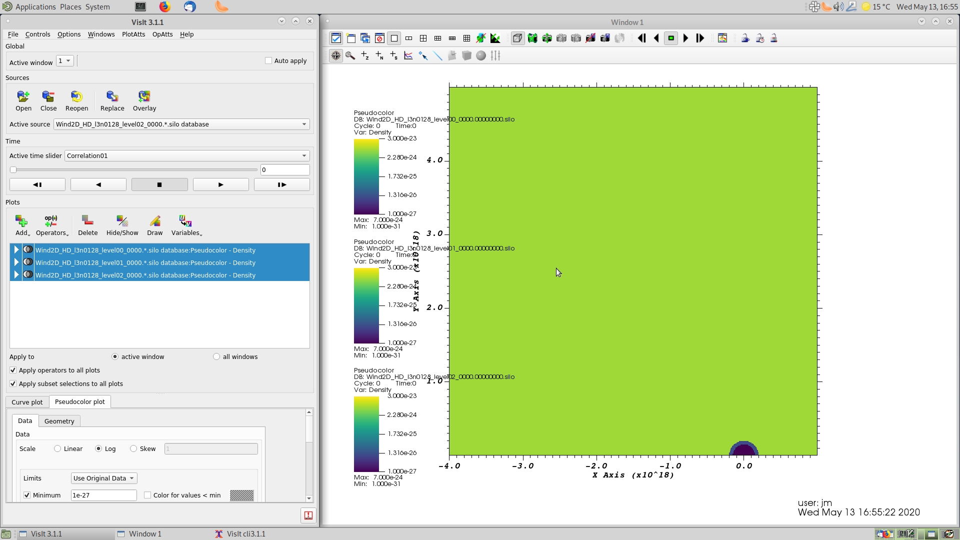
Fig. 2.4 Screenshot showing VisIt display of 2D Wind simulation at \(t=0\).

The wind is expanding radially at 1500 km/s, whereas the ISM is moving from right to left at 25 km/s. The ISM density is much larger than the wind density, however, and so the ram-pressure balance occurs at about \(z=0.5\times10^{18}\,\mathrm{cm}\). We expect to see a bow shock developing in the positive x direction, and a low-density wake forming in the negative direction. This is shown in Fig. 2.5 about 2/3 of the way through the simulation, and in Fig. 2.6 a bit later in time with a Reflect operator added to the plot to show both half-planes.

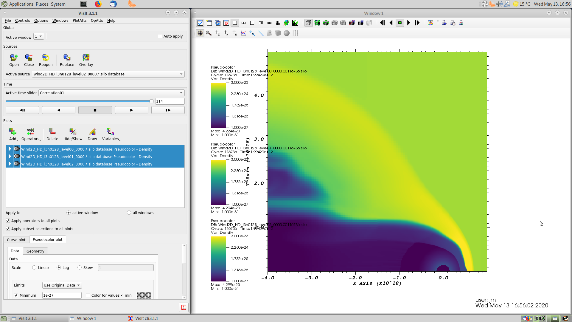
Fig. 2.5 Screenshot showing VisIt display of 2D Wind simulation at \(t\approx2\times10^{12}\,\mathrm{s}\).

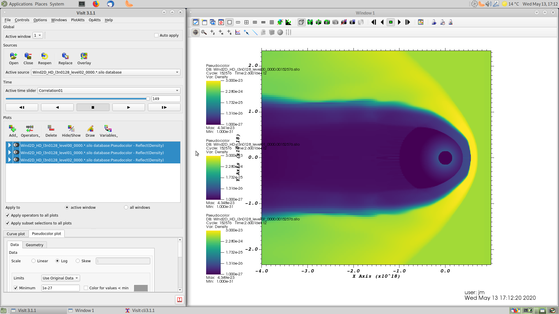
Fig. 2.6 Screenshot showing VisIt display of 2D Wind simulation at \(t\approx2.6\times10^{12}\,\mathrm{s}\), with reflection about the symmetry axis. Not all of the simulation domain is shown.

VisIt has many different types of plots and options, but for inspecting ongoing simulations the simple Pseudocolor plot is very useful. If you select all three plots in the Plots window, then click the Variables button, then you can change variables and plot any of the scalars calculated by PION, plus the gas temperature. You may need to change the Pseudocolor Attributes (Log->Lin, change max/min limits) to see useful information for the other variables. If you click File->Refresh file list from the top menus, then the time slider will update with any new files that have been saved and you can step forward to new timesteps.